

Before diving into the post - I know it is rather a late-night drop but thanks to you dear reader. Also, right as I was about to publish it, I realized it is the auspicious day of Ganesh Chaturthi today. I personally cannot think of a better day to start out on this journey and so I had to stick to the promised day! Happy Ganesh Chaturthi and Happy Reading!
If you take any college-level Intro to AI or Intro to Machine Learning class, one of the earliest concepts you will learn will be the difference between the different types of AI models - there are discriminative models and prediction models and then there are Generative models. The term “Language Models” in a more academic context can be a catch-all phrase for all of these. However, in the more popular parlance, when we talk about Language Models, we are talking about the subset of these models that is the Generative models and these are the models, dear reader, I will be talking about today.
Going back to 2015, most people would know of Jarvis - the omnipresent, know-it-all AI sidekick to Iron Man. That was something of a dream for technologists and non-technologists alike. Then in June 2020, OpenAI released GPT-3 and changed the world forever…or at least you would think so. The release of GPT-3 and EVERYTHING that came after it is a culmination of a decades-long journey in the field of Artificial Intelligence and more specifically in the field of Natural Language Processing. Now I, for one, am completely enamoured by AI (obviously, since I’m writing this really long post, and I’m assuming, to some degree, you are as well because you chose to read it) and so, for me, this is a story of true human ingenuity and perseverance and a relentless pursuit of the wondrous goal of Artificial General Intelligence.
Quick Diversion: Please subscribe to my newsletter if you would like to join me on this learning journey. Thanks!!!
So, let’s segue into this wonderful, mathematical story of how we got to ChatGPT and Llama, Claude etc., and where we are headed from here in this series on Language models. Fair warning, this will get long and mathematical but I will try my best to make it balanced for the non-technical reader.
1: The Early Days - Statistical Foundations
In the early days of computing, Claude Shannon introduced Information Theory in his seminal paper “A Mathematical Theory of Communication”1 which, in turn, led to the creation of what we now call N-gram models. Building on Shannon's work, researchers in the 1990s developed Statistical Language Models (SLMs). These models addressed contextually relevant properties of natural language from a probabilistic statistical perspective. The essence of statistical language modelling lies in ascertaining the probability of a sentence occurring within a text.
For example, consider the sentence "The quick brown fox jumps over the lazy dog". The goal of an SLM would be to calculate the probability P(S) of this sentence appearing in a text:
P(S) = P(the, quick, brown, fox, jumped, over, the, lazy, dog) = P(the) · P(quick | the) · P(brown | the quick) · P(fox | quick brown) · P(jumped | brown fox) · P(over | fox jumped) · P(the | jumped over) · P(lazy | over the) · P(dog | the lazy)
Where P(the) represents the probability of the word "the" appearing, and P(quick | the) stands for the probability of "quick" appearing given that "the" has appeared, and so on.
We typically estimate these probabilities using Maximum Likelihood Estimation (MLE), which lets us estimate probabilities based on the frequency of each word given a sufficiently large sample size.
N-Gram Models:
N-gram models, first formalized in the 1990s are a popular implementation of SLMs. These arise out of the fundamental problem that language is creative and thus, there is no good enough way to estimate probability given just the frequency of words and sentences. This is where N-Grams come in. They provide a smarter way of estimating this probability for words or even sequences of words given their history in a given corpus.2
An n-gram is essentially a contiguous sequence of n “words” from a given sample of text. The n-gram model assumes that the probability of a word depends only on the previous n-1 words.
So, in a sequence of n words, represented as:
We can compute the probability of each of the words as:
This probability is based on applying the chain rule of probabilities to decompose the probabilities of the entire sequence. But, we run into a very major problem here - we don’t really know how to compute these individual probabilities given the frequency of each word in our text. This is why we make approximations on the history of each word based on just the last few words.3 Such an assumption is called a Markov Assumption. Now, working through this assumption for a bi-gram model, we get the counts of each word from our corpus and normalize them to values between 0 and 1.4
Therefore, if we consider a bi-gram model, we can estimate the frequency using the following equation:
We can further simplify this as follows:
We can do this by equalizing the denominators in both of these equations because each occurrence of the (n-1)th word must be followed by some word, which in turn contributes to exactly one bigram count.
This is the foundation of the N-Gram models. An important note here is that the “N” represents the order of the context window. Based on this, there are the following different orders of N-Gram models.
Uni-gram Model (N=1): A Uni-gram model considers each word independently, without any context. It simply uses the frequency of individual words in the training corpus to predict probabilities. Example: P(fox, jumped, over) = P(fox) * P(jumped) * P(over)
Bi-gram Model (N=2): A Bi-gram model considers the previous word as context when predicting the next word. It uses the conditional probability of a word given the preceding word. Example: P(the, quick, brown) = P(the) * P(quick|the) * P(brown|quick)
Tri-gram Model (N=3): Tri-gram models use the previous two words as context. They provide a balance between capturing more context and maintaining computational feasibility. Example: P(the, quick, brown, fox) = P(the) * P(quick|the) * P(brown|the quick) * P(fox|quick brown)
Higher-order N-grams: Models where N > 3 are less common due to data sparsity and computational costs, but they can capture longer-range dependencies in certain applications. Example (4-gram): P(the, quick, brown, fox, jumped) = P(the) * P(quick|the) * P(brown|the quick) * P(fox|the quick brown) * P(jumped|quick brown fox)
Each increase in the order of the n-gram model allows it to capture more context, potentially improving accuracy, but at the cost of increased complexity and data requirements. The choice of which n-gram model to use often depends on the specific task, the amount of available training data, and computational constraints.
In the early days, these models were used for tasks such as speech recognition, machine translation, spell-checks, and even in page-rank operations for early web browsers. But they didn’t come without their own set of limitations. SLMs cannot understand the true meanings of words and contexts, have very limited context windows, cannot be generalized, and very importantly get incredibly complex as “N” increases.
These limitations set the stage for the next phase in the evolution of language models. Researchers began to look towards more sophisticated approaches that could capture deeper linguistic patterns and semantic relationships. This quest would lead to the neural network revolution, opening up new frontiers in language modelling and natural language processing.
2 The Neural Network Revolution:
Neural Language Models
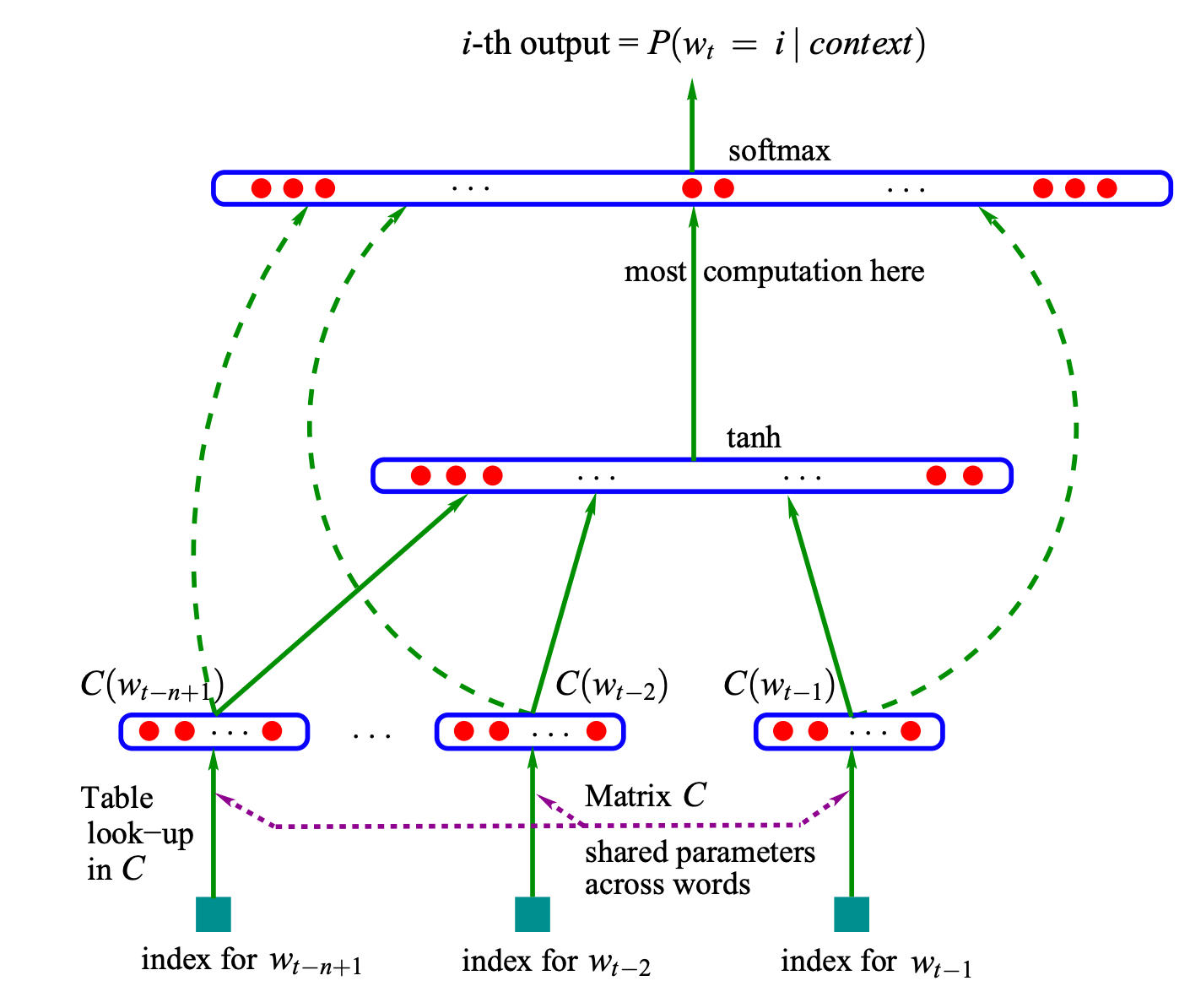
As we entered the 21st century, the field of language modelling took a significant leap forward with the introduction of Neural Language Models (NLMs) in the paper “A Neural Probabilistic Language Model” by Bengio et al in 2003. These models leveraged neural networks to predict the probabilities of word sequences, effectively handling longer sequences and mitigating the limitations associated with SLMs.
Distributed Word Representations: Each word i in the vocabulary V is associated with a feature vector C(i) ∈ ℝ^m, where m is the dimension of the feature space. Here, the mapping C is learned during training, allowing the model to discover semantic relationships between words - something SLMs could not do.
Neural Network Architecture: The model used a neural network to estimate word probabilities based on the context.
Joint Learning: The model learned word representations simultaneously with the language model parameters.
Let’s dive into some of the other key features of these models:
Probability Estimation Function: The core of these models remains estimating the probability of a word
w_tbased on the context of thet-1words that came before it. This is represented in the form of the following equation:5\(P(w_1, ..., w_T) = \prod_{t=1}^T P(w_t | w_1^{t-1})\)The most fundamental difference between the Neural models and Statistical models is in the way they estimate this probability. Instead of using count-based probability estimation like in SLMs, NLMs use a function
f(x: a neural network)to estimate this probability based on word embeddings as shown in the following equation:\( P(w_t | w_1^{t-1}) \approx f(w_t, w_{t-1}, ..., w_{t-n+1})\)These models work better because their underlying neural networks can easily handle longer sentences and mitigate the limitations of context windows, generalization, and dimensionality with increased “N” faced by SLMs more effectively.
Neural Network Architecture: Bengio et al proposed two Neural Network architectures in their papers:
Direct Architecture:
\(f(i, w_{t-1}, ..., w_{t-n+1}) = g(i, C(w_{t-1}), ..., C(w_{t-n+1}))\)In this architecture, g is a neural network that takes the context word embeddings
C(w_j)and outputs a probability distribution over the vocabulary for the next word.Cycling Architecture:
\(f(w_t, w_{t-1}, ..., w_{t-n+1}) = \frac{\exp(h(C(w_t), C(w_{t-1}), ..., C(w_{t-n+1})))}{\sum_j \exp(h(C(j), C(w_{t-1}), ..., C(w_{t-n+1})))}\)This more complex architecture uses a function h to compute a score for each possible next word, then normalizes these scores using the softmax function (the exponential terms) to get a probability distribution.
Training Objective: The following is the objective function for training the neural model. It aims to maximize the log-likelihood of the training data (the sum term) while also including a regularization term R(θ) to prevent overfitting. The 1/T term normalizes by the sequence length.
\(L = \frac{1}{T} \sum_t \log f(w_t, w_{t-1}, ..., w_{t-n+1}) + R(\theta)\)
Interestingly, these Neural Network based architectures address some of the fundamental problems faced by SLMs in the following way:
Curse of Dimensionality: By using distributed representations, the model can generalize to unseen word combinations. Similar words have similar vectors, allowing the model to make sensible predictions even for rare or unseen contexts.
Semantic Understanding: The learned word embeddings capture semantic relationships. Words with similar meanings or grammatical roles end up close in the vector space.
Longer Contexts: The neural network can effectively process longer contexts without the exponential growth in parameters that plagues n-gram models.
Non-linear Compositions: The use of non-linear activation functions allows the model to capture complex relationships between words and their contexts.
These advances allowed NLMs to significantly outperform N-gram models by reducing their perplexity6 by 20-35% on benchmark datasets. However, these models came with their own set of challenges - namely:
Computational Complexity: Training neural networks on large vocabularies and datasets was computationally intensive.
Long-range Dependencies: While better than n-grams, these models still struggled with very long-range dependencies.
Vanishing Gradients: Deep neural networks faced the vanishing gradient problem during training, limiting their ability to learn from long sequences.
At this point, as is the dictum in engineering - each failure, and each limitation fuels the next innovation. Staying true to this, let’s dive into some more advanced models.
3 From Static to Dynamic: The Rise of Recurrent and Attention-based Models
1.3.1 Recurrent Neural Network Models
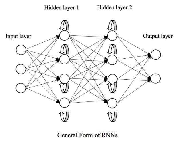
While Neural Networks improved upon n-gram models, they still struggled with variable-length inputs and capturing long-range dependencies. Recurrent Neural Networks7 (RNNs) emerged as a solution to this problem.
The core idea behind RNNs is to use the same set of weights repeatedly across different time steps of the input sequence. This weight sharing allows the network to process sequences of arbitrary length while keeping the number of parameters constant.8
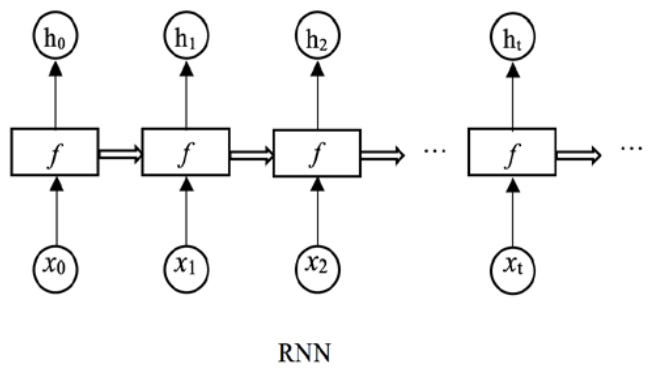
We can define an RNN using the following equation:
Where:
We can visualize RNNs as a chain of repeating modules in the following manner:
In our context of Language Models, Recurrent Neural Networks offer several advantages:
Variable-length inputs: RNNs could handle sentences of different lengths naturally.
Shared parameters: The same weights are used at each time step, allowing the model to generalize across positions in the sequence.
Theoretical ability to capture long-range dependencies: In principle, information could be propagated through many time steps.
For an RNN based Language Model, the probability estimation for the next word prediction task then becomes:
Where h_t is the hidden state after processing words w_1 through w_{t-1}.
Now, RNNs could, in theory, capture dependencies of arbitrary length. However, they faced the vanishing gradient problem during training, limiting their effectiveness for long sequences.
1.3.2 Long Short-Term Memory Networks:
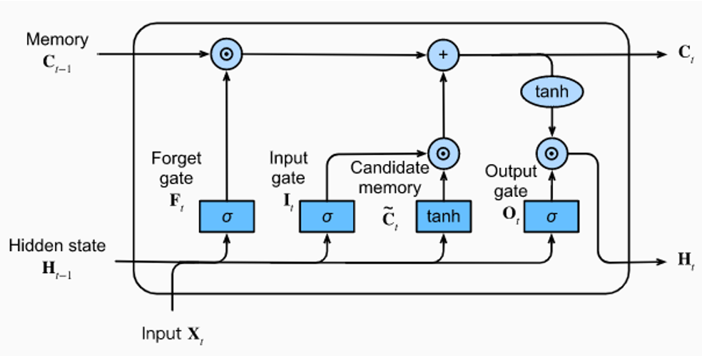
To address the vanishing gradient problem, Hochreiter and Schmidhuber introduced Long Short-Term Memory (LSTM) networks in 1997. LSTMs became widely adopted for language modelling in the early 2010s.
LSTM Architecture
The LSTM introduces a memory cell and gates to control information flow:
Where,
LSTMs were better able to capture long-range dependencies and became the standard for many sequence modelling tasks, including language modelling.
The architectural improvements brought along by RNNs and LSTMs were also accompanied by significant improvements in learning word representations and attention mechanisms, which would go on to become fundamental to Language model improvements in the future.
These are both deep, deep rabbit holes on their own so I will only make brief notes on them here, but they are topics of their own that will deserve to be discussed on their own.
1.3.3 Word Embeddings and Transfer Learning:
Word2Vec
Mikolov et al. introduced Word2Vec9 (Ilya Sutskever is one of the authors of this paper!!!) in 2013, which efficiently learned high-quality word embeddings. The Skip-gram model, one of the Word2Vec architectures, aims to predict context words given a target word:
where,
These embeddings captured semantic relationships between words and could be used to initialize the word representations in more complex language models.
1.3.4 Attention Mechanisms:
While LSTMs improved upon vanilla RNNs, they still struggled with very long sequences. Attention mechanisms, introduced by Bahdanau et al. in 2014, allowed models to focus on relevant parts of the input sequence when generating each output.
In traditional sequence-to-sequence models, the entire input sequence was compressed into a fixed-size vector, which was then used to generate the output. This approach struggled with long sequences, as it was difficult to encode all necessary information into a single vector.
Attention mechanisms address this by allowing the model to focus on different parts of the input sequence at each step of the output generation. This mimics human cognition - when we process language, we don't consider every word with equal importance at every moment.
Basic Attention Mechanism:
The basic attention mechanism can be described as follows:
For each output step, the model computes a set of attention weights.
These weights determine how much focus to place on different parts of the input sequence.
The model then uses these weighted inputs to generate the output.
We can express this mathematically as10:
where,
Attention mechanisms had a significant and long-lasting impact on language modelling:
They improved the handling of long-range dependencies by allowing direct connections between distant states, attention mitigated the vanishing gradient problem that plagued RNNs.
They increased interpretability as the attention weights provide insight into which parts of the input the model is focusing on, making the model's decision-making process more transparent.
They allowed for better parallelization because unlike RNNs, which process sequences step by step, attention mechanisms allow for more parallel computation.
They lay the foundation for Transformers which would go on to revolutionize NLP.
As the power of attention mechanisms became apparent, researchers developed several variants to further enhance their capabilities:
Soft vs. Hard Attention: While the original attention mechanism used a "soft" approach, calculating weighted averages over all input states, researchers also explored "hard" attention. This variant selects a single input state, potentially offering more focused and interpretable results, albeit at the cost of being non-differentiable and thus more challenging to train.11
Self-Attention: A crucial development in attention mechanisms was the concept of self-attention, where a sequence attends to itself. This allows the model to capture intra-sequence dependencies without the need for recurrent connections. Self-attention would become a cornerstone of the Transformer architecture, which we'll explore in the next chapter.12
Multi-Head Attention: Building upon self-attention, multi-head attention allows the model to attend to different parts of the sequence in different ways simultaneously. This multi-faceted approach enables the model to capture various types of relationships within the data, from syntactic to semantic dependencies.13
These advancements in attention mechanisms set the stage for a paradigm shift in language modelling. By allowing models to focus dynamically on relevant parts of the input, attention mechanisms addressed many of the limitations of previous architectures. However, the full potential of attention was yet to be realized. In the next part, I’ll discuss how these ideas culminated in the Transformer architecture, leading to the rise of large pre-trained language models that have revolutionized the world.
4 The Transformer Revolution
1.4.1 The Architecture:
In 2017, Vaswani et al. introduced the Transformer model in their groundbreaking paper "Attention Is All You Need"14. This architecture marked a paradigm shift in natural language processing, eschewing recurrence and convolutions entirely in favour of attention mechanisms. Let's delve into the key components and innovations of the Transformer.
The fundamental building block of the Transformer is the self-attention mechanism. Unlike previous sequence transduction models that used complex recurrent or convolutional neural networks, the Transformer relies solely on attention to draw global dependencies between input and output.
The self-attention mechanism allows the model to attend to different parts of the input sequence for each element of the output sequence. Mathematically, it can be described as:
Where Q, K, and V are query, key, and value matrices, respectively, and $d_k$ is the dimension of the key vectors.
To enhance the model's ability to focus on different positions, the authors introduced multi-head attention (I briefly mentioned this in the previous section). This allows the model to jointly attend to information from different representation subspaces at different positions. We can define multi-head attention as:
where we compute each head as:
Within this, each layer in the encoder and decoder contains a fully connected feed-forward network, applied to each position separately and identically as:
Since the model contains no recurrence or convolution, positional encodings are added to the input embeddings to provide information about the relative or absolute position of the tokens in the sequence:
Where:
pos is the position of the token in the sequence
i is the dimension
d_model is the dimensionality of the model's embeddings
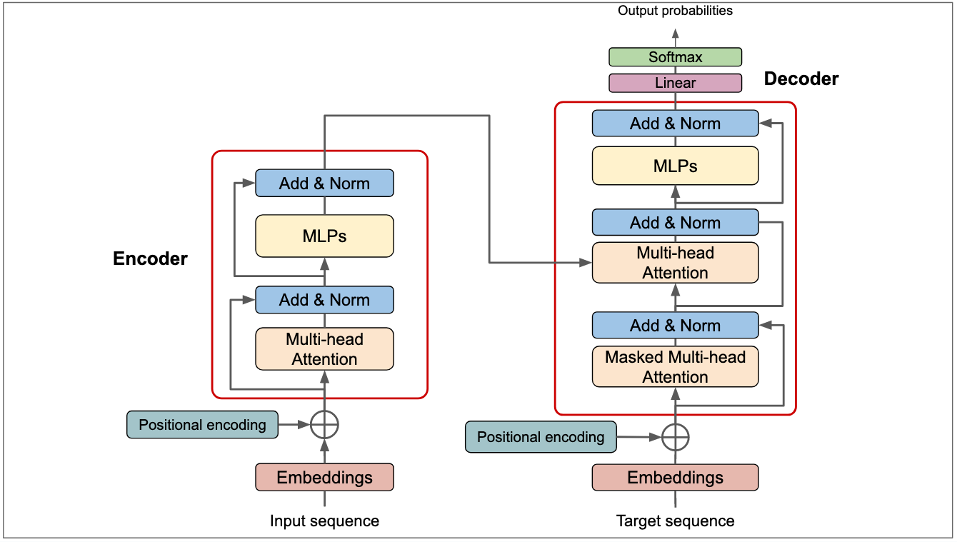
Putting it all together, what we get is an encoder-decoder structure such that:
Encoder: Composed of a stack of N identical layers, each with two sub-layers:
Multi-head self-attention mechanism
Position-wise fully connected feed-forward network
Decoder: Also composed of N identical layers, but with an additional sub-layer that performs multi-head attention over the encoder stack's output.
1.4.2 Advantages of the Transformer:
The transformer removes recurrence and therefore, allows for significantly improved parallelization during training.
The self-attention mechanism allows the model to easily learn the long-range dependencies in the data.
For sequence transduction tasks15, the Transformer can be faster to train than architectures based on recurrent or convolutional layers.
The attention distributions from the model can be visualized and interpreted, providing insights into its decision-making process.
A true testament to the revolutionary nature of the Transformer is its versatility. Not only is it fantastic at Machine Translation tasks (example: Google Translate), it was also demonstrated by the authors that the Transformer is also effective at English constituency parsing tasks.16
1.4.3 Some really cool applications:
The introduction of the Transformer architecture has revolutionized not just machine translation, but a wide array of NLP tasks and beyond.
Transformer-based models have significantly improved the quality and fluency of machine translation. Google Translate, for instance, adopted Transformer models, leading to more accurate and contextually appropriate translations. This has made it easier for people to communicate across language barriers, whether for business, travel, or cultural exchange.
Transformer models have dramatically improved chatbots and virtual assistants, making them more contextually aware and capable of maintaining coherent conversations (While the Transformer did have a large impact on these, it was not until the advent of Large Language Models that these tasks were truly revolutionized).
5 Conclusion
As we approach the end of this very long post, I hope I have done justice in covering the history of Language Models and I hope, you dear reader, can gain something out of this. I know this has been very verbose but I sincerely thank you for sticking till the end (if you did) and bearing with me.
In part 2, I am excited to really dive deeper into the exciting stuff and venture into the realm of Language Models as they exist today. How and why they do what they do and how they are truly a marvel of some really ingenious human engineering.
Personal Note and Acknowledgment:
I did not expect anyone to even get to this but if you, dear reader, did - at the risk of being repetitive I thank you for reading this post and supporting me. If you liked this post, please like and share it
with your friends if you can. Most importantly, I truly hope I was able to provide some value to you.
To quote Andrej Karpathy:
Learning is not supposed to be fun. It doesn't have to be actively not fun either, but the primary feeling should be that of effort. It should look a lot less like that "10 minute full body" workout from your local digital media creator and a lot more like a serious session at the gym.
It is also important I thank Spotify and very importantly a great man called Pyotr Ilyich Tchaikovsky (Shoutout to the 1812 Overture) because, without these two, I would have never been able to finish this!!
My attempt through this blog is to do the heavy lifting so that I can make the learning process a little easier for myself and you. This is why, I am really excited to have you join me on this journey. If you have any feedback for me, please leave a comment.
Claude E. Shannon, “A Mathematical Theory of Communication,” The Bell System Technical Journal 27 (October 1948): 623–56, https://doi.org/10.1109/9780470544242.ch1.
1. Daniel Jurafsky and James H. Martin, N-gram language models, August 20, 2024, https://web.stanford.edu/~jurafsky/slp3/3.pdf.
Ibid
Normalizing in this context means dividing by the total count so the resulting probabilities fall between 0 and 1 and sum to 1.
Yoshua Bengio, Réjean Ducharme, and Pascal Vincent, "A Neural Probabilistic Language Model," Advances in Neural Information Processing Systems 12 (2000): 932-938.
Perplexity is a measure of how well a model predicts a sequence of words.
ODSC Community, “Understanding the Mechanism and Types of Recurrent Neural Networks,” Open Data Science - Your News Source for AI, Machine Learning & more, March 5, 2021, https://opendatascience.com/understanding-the-mechanism-and-types-of-recurring-neural-networks/.
Ibid
Mikolov, Tomas, Ilya Sutskever, Kai Chen, Greg Corrado, and Jeffrey Dean. “Distributed Representations of Words and Phrases and Their Compositionality.” arXiv.org, October 16, 2013. https://arxiv.org/abs/1310.4546.
Dzmitry Bahdanau, Kyunghyun Cho, and Yoshua Bengio, “Neural Machine Translation by Jointly Learning to Align and Translate,” arXiv.org, May 19, 2016, https://arxiv.org/abs/1409.0473.
“Must-Read Starter Guide to Mastering Attention Mechanisms in Machine Learning,” Arize AI, June 12, 2023, https://arize.com/blog-course/attention-mechanisms-in-machine-learning/.
Ibid
Ashish Vaswani et al., “Attention Is All You Need,” arXiv.org, August 2, 2023, https://arxiv.org/abs/1706.03762v7.
Ibid
Sequence transduction tasks refer to problems in which a model converts an input sequence into an output sequence.
English constituency parsing is a natural language processing (NLP) task that involves analyzing the syntactic structure of a sentence and breaking it down into subcomponents, or "constituents." The goal of constituency parsing is to generate a parse tree that represents the hierarchical structure of a sentence according to a formal grammar, typically based on context-free grammars (CFGs).